Consensus, moved a fraction of the way toward the forecast
The customer’s question is never “what will revenue be?” — they already have consensus. It is “where is consensus wrong?” This page builds the number that answers it, and shows every step with real figures.
The worked example’s numbers are also a golden test, so this page and the library cannot drift apart.
Step 1 — the inputs, and when they may be used
Four inputs per company-quarter, each read as of the moment the number is published: the value whose known_at is the latest one strictly before that instant.
Five steps, every one explicit: anchor, reshape, age, measure the revision, join it on. A method never reaches past this pipeline to the raw panel.
Step 3 — the three ingredients
All three are relative quantities, so companies of any size are comparable.
With the model forecast \(m\), the consensus \(c\), the consensus \(c_{-30}\) read thirty days earlier, and the actual \(y\) (symbols as on the notation page):
\[
\Delta = \frac{m - c}{\lvert c\rvert}
\qquad\text{the gap: what the data says consensus is missing}
\]
\[
r = \frac{c}{c_{-30}} - 1
\qquad\text{the revision: what analysts have already started to do}
\]
\[
s = \frac{y}{c} - 1
\qquad\text{the surprise: the target, known only afterwards}
\]
The revision is two anchored reads of the same quantity, thirty days apart, which is why it lives in history and not in the method. A missing prior consensus comes back missing, never as a revision of zero — those are different facts.
Step 4 — fit the weights once, and freeze them
The published estimate is a forecast of the surprise from the gap and the revision:
\[
\hat s = a + b_\Delta\, \Delta + b_r\, r
\]
The customary beat \(a\) is the surprise when the gap and the revision are both zero. The gap weight \(b_\Delta\) and the revision weight \(b_r\) say how much of each carries into the expected surprise \(\hat s\).
Fitted by ordinary least squares on reports before a cut-off date, then never refitted inside the evaluation period. The library ships the fitted sets as data:
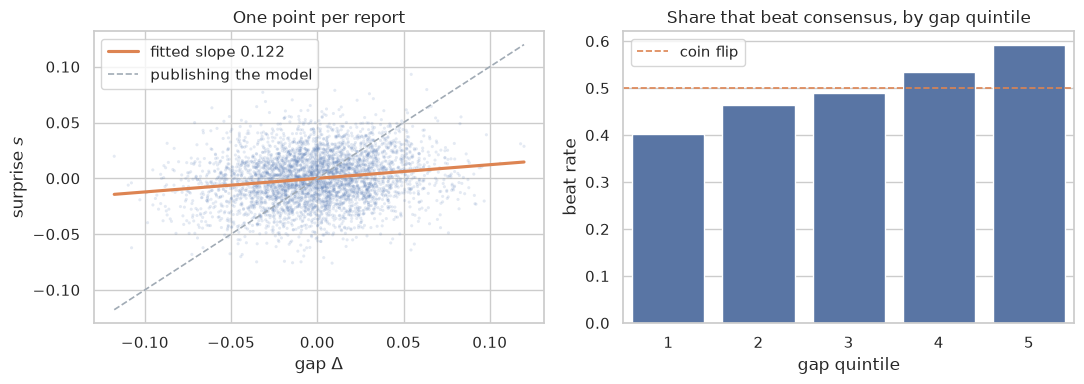
This is the step that surprises people. Let \(\xi\) be the part of the surprise that is genuinely knowable in advance. The gap \(\Delta\) is a noisy reading of it, with noise \(\eta\), and the surprise \(s\) is \(\xi\) plus what nobody could have known, \(\zeta\):
A signal-to-total-variance ratio, always between 0 and 1: the classical attenuation from measurement error (Fuller 1987). A weight of 0.129 does not mean the model is usually wrong. It means the gap’s noise variance \(\operatorname{Var}(\eta)\) is about seven times \(\operatorname{Var}(\xi)\), the variance of its predictive part.
Figure 1: Simulated from the attenuation formula with the shipped noise ratio. The cloud is wide, the line is shallow, and the quintile sort is still monotone — which is the whole business case.
Why \(b_r\) is above 1
A coefficient above one looks wrong and is not. Analysts revise toward the truth but stop short, so the observed revision is a partial adjustment (Abarbanell and Bernard 1992; Gleason and Lee 2003). Revisions therefore predict later forecast errors (Coibion and Gorodnichenko 2015; Bouchaud et al. 2019). The regression recovers the structural weight divided by the share analysts complete. A weight of 1.28 implies they complete roughly three-quarters of the move before the report.
Step 5 — anchor
Do not publish the expected surprise \(\hat s\) as a level on its own. Multiply consensus \(c\) by it to get the anchored level \(\hat y\):
\[
\hat y = c \times (1 + \hat s)
\]
Substituting the gap shows what anchoring really is:
\[
\hat y = \underbrace{c\,(1 + a + b_r r)}_{\text{consensus, corrected}}
+ \underbrace{b_\Delta\,(m - c)}_{\text{a fraction of the disagreement}}
\]
The three contributions sum to the expected surprise. That is what makes the number attributable: a customer sees which part of the adjustment is alternative data and which is consensus dynamics, and each data partner sees its own contribution.
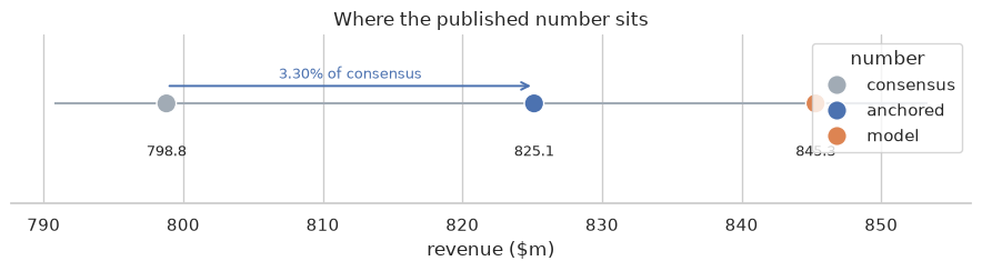
Figure 2: Where the published number sits, for the worked example.
The published number inherits the accuracy of consensus, and every bit of the alternative data sits in the difference.
Step 6 — publish nothing rather than a fallback
A feed that fills a gap with consensus is publishing “no information” as if it were a forecast. A feed that drops the row silently makes the gap invisible. So the row stays, the numbers go missing, and the reason travels with it.
The check order is part of the contract: missing input, then stale model, then stale consensus, then wide gap. A subject that is both stale and wide-gapped reports the staleness, because that is the fault to fix.
An absolute gap at or above the shipped 25% limit is almost always a mismatched fiscal period or a restatement rather than information, which is why it is a data break and not a very strong signal.
Step 7 — version every value
Fitted coefficients become constants shipped with the signal, re-estimated on a schedule and never tuned between releases. A consumer who backtests your history needs to know which coefficient set produced each published value.
Show the code
pd.DataFrame( [ {"version": parameters.version,"fitted_through": str(parameters.fitted_through),"expected_surprise": f"{out.expected_surprise:+.4%}","anchored_level": f"{out.anchored_level:,.2f}", }for parameters in (pf.ANCHORING_2025_01, pf.CORE_2025_01)for out in [ pf.AnchoredEstimate(forecast_source="model", parameters=parameters) .fit(subjects) .apply(subjects) .iloc[0] ] ])
version
fitted_through
expected_surprise
anchored_level
0
anchoring-2025-01
2024-12-31
+3.2968%
825.13
1
core-2025-01
2024-12-31
+2.5228%
818.95
Same inputs, different published number, and the difference is explainable rather than mysterious. The record a run writes down carries both:
Plain values only. It serialises with nothing more than a JSON dump, and no pickle stands between a published number and its explanation.
What to take away
The arithmetic is ten lines. Everything that makes it a product is around it.
Point-in-time is a property of the read, not the formula.
The gap weight is an attenuation ratio. 0.129 says the gap is noisy, not that the model is wrong.
Publish nothing rather than a fallback, and emit the reason.
A parameter set is data with a version.
Next: the Bayesian posterior, which reaches a similar number by a different route and carries an uncertainty band.
References
Abarbanell, Jeffery S., and Victor L. Bernard. 1992. “Tests of Analysts’ Overreaction/Underreaction to Earnings Information as an Explanation for Anomalous Stock Price Behavior.”The Journal of Finance 47 (3): 1181–207. https://doi.org/10.1111/j.1540-6261.1992.tb04010.x.
Bartov, Eli, Dan Givoly, and Carla Hayn. 2002. “The Rewards to Meeting or Beating Earnings Expectations.”Journal of Accounting and Economics 33 (2): 173–204. https://doi.org/10.1016/S0165-4101(02)00045-9.
Bouchaud, Jean-Philippe, Philipp Krüger, Augustin Landier, and David Thesmar. 2019. “Sticky Expectations and the Profitability Anomaly.”The Journal of Finance 74 (2): 639–74. https://doi.org/10.1111/jofi.12734.
Coibion, Olivier, and Yuriy Gorodnichenko. 2015. “Information Rigidity and the Expectations Formation Process: A Simple Framework and New Facts.”American Economic Review 105 (8): 2644–78. https://doi.org/10.1257/aer.20110306.
Gleason, Cristi A., and Charles M. C. Lee. 2003. “Analyst Forecast Revisions and Market Price Discovery.”The Accounting Review 78 (1): 193–225. https://doi.org/10.2308/accr.2003.78.1.193.
Granger, Clive W. J., and Ramu Ramanathan. 1984. “Improved Methods of Combining Forecasts.”Journal of Forecasting 3 (2): 197–204. https://doi.org/10.1002/for.3980030207.
Richardson, Scott, Siew Hong Teoh, and Peter D. Wysocki. 2004. “The Walk-down to Beatable Analyst Forecasts: The Role of Equity Issuance and Insider Trading Incentives.”Contemporary Accounting Research 21 (4): 885–924. https://doi.org/10.1506/KHNW-PJYL-ADUB-0RP6.