Anchoring a data-driven estimate on consensus

Consensus, moved a fraction of the way toward the forecast

The customer’s question is never “what will revenue be?” — they already have consensus. It is “where is consensus wrong?” This page builds the number that answers it, and shows every step with real figures.

NoteProvenance

Ported from docs/anchoring.qmd and docs/anchoring_signal.py in the buy-side consensus repository, from one company-quarter of scalars to the panel API. That reference ends in a self-check with real numbers, and the self-check is a golden test here, so this page and the published research cannot drift apart.

Step 1 — the inputs, and when they may be used

Four inputs per company-quarter, each read as of the moment the number is published: the value whose known_at is the latest one strictly before that instant.

Input Cap
model at most 21 days old
consensus at most 60 days old
consensus 30 days earlier at most 60 days old
first reported actual evaluation only, never an input
Show the code
AS_OF = pd.Timestamp("2026-01-20", tz="UTC")
LOOKBACK = pd.Timedelta(days=30)

estimates = pfc.validate_estimates(pf.example_panel())
estimates
entity period target period_end source value known_at
0 ZS 2026Q1 revenue 2026-01-31 00:00:00+00:00 consensus 790.0 2025-12-01 00:00:00+00:00
1 ZS 2026Q1 revenue 2026-01-31 00:00:00+00:00 consensus 798.8 2026-01-15 00:00:00+00:00
2 ZS 2026Q1 revenue 2026-01-31 00:00:00+00:00 model 845.3 2026-01-12 00:00:00+00:00

Two consensus prints, one model run. The older consensus is what the 30-day revision measures against.

Step 2 — read it, reshape it, age it

Show the code
anchored = pfc.latest_before(estimates, AS_OF)
subjects = pfc.age_at(pfc.pivot_sources(anchored), AS_OF)
revisions = pfc.consensus_revision(estimates, AS_OF, lookback=LOOKBACK)
subjects = subjects.merge(revisions, on=pfc.subject_index(subjects), how="left")
subjects[["entity", "consensus", "model", "consensus_revision", "model_age", "consensus_age"]]
entity consensus model consensus_revision model_age consensus_age
0 ZS 798.8 845.3 0.011139 8 days 5 days

Five steps, every one explicit: anchor, reshape, age, measure the revision, join it on. A method never reaches past this pipeline to the raw panel.

Step 3 — the three ingredients

All three are relative quantities, so companies of any size are comparable.

\[ g = \frac{\text{model}}{\text{consensus}} - 1 \qquad\text{the gap: what the data says consensus is missing} \]

\[ r = \frac{\text{consensus}_t}{\text{consensus}_{t-30}} - 1 \qquad\text{the revision: what analysts have already started to do} \]

\[ s = \frac{\text{actual}}{\text{consensus}} - 1 \qquad\text{the surprise: the target, known only afterwards} \]

The revision is two anchored reads of the same quantity, thirty days apart, which is why it lives in history and not in the method. A missing prior consensus comes back missing, never as a revision of zero — those are different facts.

Step 4 — fit the weights once, and freeze them

The published estimate is a forecast of the surprise from the gap and the revision:

\[ \hat s = a + b_g\, g + b_r\, r \]

Fitted by ordinary least squares on reports before a cut-off date, then never refitted inside the evaluation period. The library ships the fitted sets as data:

Show the code
pd.DataFrame(
    [
        pfc.STUDY_2025_01.model_dump(mode="json"),
        pfc.CORE_2025_01.model_dump(mode="json"),
    ]
).set_index("version").T
version study-2025-01 core-2025-01
customary_beat 0.0112 0.0089
gap_weight 0.129 0.0442
revision_weight 1.28 1.2348
maximum_absolute_gap 0.25 0.25
maximum_prediction_age P21D P21D
maximum_consensus_age P60D P60D
fitted_through 2024-12-31 2024-12-31

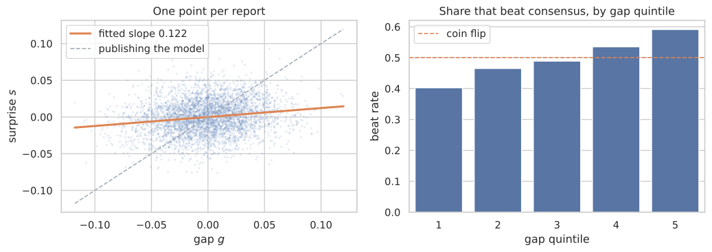
Why \(b_g\) is near 0.13 and not 1

This is the step that surprises people. Let \(\theta\) be the part of the surprise that is genuinely knowable in advance. The gap is a noisy reading of it, and the surprise is \(\theta\) plus what nobody could have known:

\[ g = \theta + \eta, \qquad s = \theta + \epsilon \]

\[ b_g = \frac{\operatorname{Cov}(s, g)}{\operatorname{Var}(g)} = \frac{\operatorname{Var}(\theta)}{\operatorname{Var}(\theta) + \operatorname{Var}(\eta)} \]

A signal-to-total-variance ratio, always between 0 and 1. A weight of 0.129 does not mean the model is usually wrong. It means the gap’s noise variance is about seven times the variance of its predictive part.

Show the code
rng = np.random.default_rng(20260922)
size = 4000
theta = rng.normal(0, 0.012, size)
reports = pd.DataFrame(
    {
        "gap": theta + rng.normal(0, 0.012 * np.sqrt(6.75), size),
        "surprise": theta + rng.normal(0, 0.020, size),
    }
)
slope = np.cov(reports.surprise, reports.gap)[0, 1] / reports.gap.var()
reports["quintile"] = pd.qcut(reports.gap, 5, labels=[1, 2, 3, 4, 5])

figure, axes = plt.subplots(1, 2, figsize=(11, 4))
sns.regplot(
    data=reports, x="gap", y="surprise", ax=axes[0], ci=None,
    scatter_kws={"s": 5, "alpha": 0.15, "color": pf.ACCENT, "edgecolor": "none"},
    line_kws={"color": pf.WARM, "label": f"fitted slope {slope:.3f}"},
)
grid = np.linspace(reports.gap.min(), reports.gap.max(), 50)
axes[0].plot(grid, grid, color=pf.GREY, ls="--", lw=1.2, label="publishing the model")
axes[0].set(xlabel="gap $g$", ylabel="surprise $s$", title="One point per report")
axes[0].legend()

sns.barplot(
    data=reports.assign(beat=reports.surprise > 0),
    x="quintile", y="beat", ax=axes[1], color=pf.ACCENT, errorbar=None,
)
axes[1].axhline(0.5, color=pf.WARM, lw=1.2, ls="--", label="coin flip")
axes[1].set(
    xlabel="gap quintile", ylabel="beat rate",
    title="Share that beat consensus, by gap quintile",
)
axes[1].legend()
figure.tight_layout()
Figure 1: Simulated from the attenuation formula with the study’s noise ratio. The cloud is wide, the line is shallow, and the quintile sort is still monotone — which is the whole business case.

Why \(b_r\) is above 1

A coefficient above one looks wrong and is not. Analysts revise toward the truth but stop short, so the observed revision is a partial adjustment. The regression recovers the structural weight divided by the share analysts complete. A weight of 1.28 implies they complete roughly three-quarters of the move before the report.

Step 5 — anchor

Do not publish the expected surprise as a level on its own. Multiply consensus by it:

\[ \hat y = c \times (1 + \hat s) \]

Substituting the gap shows what anchoring really is:

\[ \hat y = \underbrace{c\,(1 + a + b_r r)}_{\text{consensus, corrected}} + \underbrace{b_g\,(m - c)}_{\text{a fraction of the disagreement}} \]

Show the code
method = pfc.AnchoredEstimate(forecast_source="model")
published = method.fit(subjects).apply(subjects)
row = published.iloc[0]

pd.DataFrame(
    [
        {"field": name, "value": f"{row[name]:+.4%}"}
        for name in [*pfc.CONTRIBUTION_COLUMNS, pfc.EXPECTED_SURPRISE_COLUMN]
    ]
    + [
        {"field": pfc.ANCHORED_LEVEL_COLUMN, "value": f"{row.anchored_level:,.2f}"},
        {"field": pfc.PARAMETERS_VERSION_COLUMN, "value": row.parameters_version},
    ]
)
field value
0 contribution_customary_beat +1.1200%
1 contribution_gap +0.7509%
2 contribution_revision +1.4258%
3 expected_surprise +3.2968%
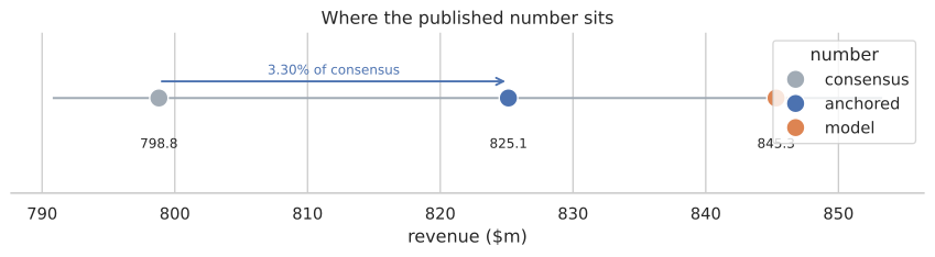
4 anchored_level 825.13
5 parameters_version study-2025-01

The three contributions sum to the expected surprise. That is what makes the number attributable: a customer sees which part of the adjustment is alternative data and which is consensus dynamics, and each data partner sees its own contribution.

Show the code
places = pd.DataFrame(
    [
        {"number": "consensus", "level": row.consensus},
        {"number": "anchored", "level": row.anchored_level},
        {"number": "model", "level": row.model},
    ]
)

figure, axis = plt.subplots(figsize=(9, 2.6))
axis.hlines(0, row.consensus - 8, row.model + 8, color=pf.GREY, lw=1.5, zorder=1)
sns.scatterplot(
    data=places, x="level", y=0, hue="number", s=160, ax=axis, zorder=3,
    palette=[pf.GREY, pf.ACCENT, pf.WARM],
)
for _, place in places.iterrows():
    axis.annotate(f"{place.level:.1f}", (place.level, -0.42), ha="center", fontsize=9)
axis.annotate(
    "", xy=(row.anchored_level, 0.14), xytext=(row.consensus, 0.14),
    arrowprops={"arrowstyle": "->", "color": pf.ACCENT, "lw": 1.4},
)
axis.annotate(
    f"{row.expected_surprise:.2%} of consensus",
    ((row.consensus + row.anchored_level) / 2, 0.2),
    color=pf.ACCENT, ha="center", fontsize=9,
)
axis.set(ylim=(-0.8, 0.55), yticks=[], ylabel="", xlabel="revenue ($m)")
axis.set_title("Where the published number sits")
sns.despine(ax=axis, left=True)
figure.tight_layout()
Figure 2: Where the published number sits, for the worked example.

The published number inherits the accuracy of consensus, and every bit of the alternative data sits in the difference.

Step 6 — publish nothing rather than a fallback

A feed that fills a gap with consensus is publishing “no information” as if it were a forecast. A feed that drops the row silently makes the gap invisible. So the row stays, the numbers go missing, and the reason travels with it.

Show the code
cases = pd.DataFrame(
    {
        "entity": ["fine", "no model", "stale model", "stale consensus", "wide gap"],
        "period": ["2026Q1"] * 5,
        "target": ["revenue"] * 5,
        "period_end": pd.to_datetime(["2026-01-31"] * 5, utc=True),
        "consensus": [798.8] * 5,
        "model": [845.3, float("nan"), 845.3, 845.3, 1100.0],
        "consensus_revision": [0.0] * 5,
        "model_age": pd.to_timedelta([8, 8, 22, 8, 8], unit="D"),
        "consensus_age": pd.to_timedelta([5, 5, 5, 61, 5], unit="D"),
    }
)
method.fit(cases).apply(cases)[
    [
        "entity",
        pfc.ELIGIBLE_COLUMN,
        pfc.ELIGIBILITY_REASON_COLUMN,
        pfc.EXPECTED_SURPRISE_COLUMN,
        pfc.ANCHORED_LEVEL_COLUMN,
    ]
]
entity eligible eligibility_reason expected_surprise anchored_level
0 fine True publishable 0.018709 813.74506
1 no model False missing_input NaN NaN
2 stale model False stale_prediction NaN NaN
3 stale consensus False stale_consensus NaN NaN
4 wide gap False gap_too_wide NaN NaN

The check order is part of the contract: missing input, then stale model, then stale consensus, then wide gap. A subject that is both stale and wide-gapped reports the staleness, because that is the fault to fix.

A gap beyond 25% is almost always a mismatched fiscal period or a restatement rather than information, which is why it is a data break and not a very strong signal.

Step 7 — version every value

Fitted coefficients become constants shipped with the signal, re-estimated on a schedule and never tuned between releases. A consumer who backtests your history needs to know which coefficient set produced each published value.

Show the code
pd.DataFrame(
    [
        {
            "version": parameters.version,
            "fitted_through": str(parameters.fitted_through),
            "expected_surprise": f"{out.expected_surprise:+.4%}",
            "anchored_level": f"{out.anchored_level:,.2f}",
        }
        for parameters in (pfc.STUDY_2025_01, pfc.CORE_2025_01)
        for out in [
            pfc.AnchoredEstimate(forecast_source="model", parameters=parameters)
            .fit(subjects)
            .apply(subjects)
            .iloc[0]
        ]
    ]
)
version fitted_through expected_surprise anchored_level
0 study-2025-01 2024-12-31 +3.2968% 825.13
1 core-2025-01 2024-12-31 +2.5228% 818.95

Same inputs, different published number, and the difference is explainable rather than mysterious. The record a run writes down carries both:
Show the code
method.fit(subjects).to_dict()
{'method': 'anchored.estimate',
 'forecast_source': 'model',
 'consensus_source': 'consensus',
 'parameters_version': 'study-2025-01',
 'fitted_through': '2024-12-31',
 'parameters': {'customary_beat': 0.0112,
  'gap_weight': 0.129,
  'revision_weight': 1.28,
  'maximum_absolute_gap': 0.25,
  'maximum_prediction_age': 'P21D',
  'maximum_consensus_age': 'P60D',
  'version': 'study-2025-01',
  'fitted_through': '2024-12-31'}}

Plain values only. It serialises with nothing more than a JSON dump, and no pickle stands between a published number and its explanation.

What to take away

  • The arithmetic is ten lines. Everything that makes it a product is around it.
  • Point-in-time is a property of the read, not the formula.
  • The gap weight is an attenuation ratio. 0.129 says the gap is noisy, not that the model is wrong.
  • Publish nothing rather than a fallback, and emit the reason.
  • A parameter set is data with a version.

Next: the Bayesian posterior, which reaches a similar number by a different route and carries an uncertainty band.