The Bayesian posterior

Three noisy readings of one unknown, weighted by how well each has done

The anchored estimate treats consensus as the anchor and moves a fixed fraction of the way toward the model. This method treats all three readings symmetrically and lets each one’s own track record decide its weight.

NoteProvenance

Ported from docs/bayesian_signal.py and docs/bayesian.qmd in the buy-side consensus repository, which follow IndependentBayesianRegularizedPredictionSignal in exabel/python/exabel/timeseries/dsl/signals/bayesian_kpi_prediction_signal.py. The reference’s self-check is a golden test here.

The setup

One unknown: \(\theta\), the company’s revenue growth for the coming quarter. Three noisy readings of it, each with its own variance.

Reading Symbol Where its variance comes from
Prior \(\mu_0\) the company’s own realised growth history
Model \(x_A\) the model’s error against realised growth
Consensus \(x_C\) consensus’s error, or analyst dispersion

The normal–normal update

Assume each reading is an independent Gaussian observation of \(\theta\). The posterior is proportional to prior times likelihoods, and collecting the exponent as a quadratic in \(\theta\) gives a Gaussian again. Writing \(\tau_i = 1/\sigma_i^2\) for precisions:

\[ \hat\theta = \frac{\mu_0\tau_0 + x_A\tau_A + x_C\tau_C}{\tau_0 + \tau_A + \tau_C}, \qquad \operatorname{Var}(\theta \mid \text{data}) = \frac{1}{\tau_0 + \tau_A + \tau_C} \]

Two structural facts follow immediately:

  • Precisions add. Every additional independent source, however weak, reduces computed posterior variance under these assumptions. Predictive accuracy can still worsen when errors are correlated or variances are misspecified.
  • Weights are precision shares. The coefficient on each source is \(\tau_i / \sum_j \tau_j\), so the three weights sum to one by construction and none can be negative.

Growth space, not level space

The method works on growth over the previous actual, not on revenue levels. Two reasons:

  • Scale. Revenue levels are non-stationary. Sequential growth is far closer to stationary, which is what makes a variance estimated over history meaningful at all.
  • The prior needs a sample. A prior on “this company’s growth” can be estimated from its own history. A prior on “this company’s revenue in dollars” cannot, without a trend model.

The inputs, measured point-in-time

history supplies the statistics, each read strictly before the moment being forecast.

Show the code
AS_OF = pd.Timestamp("2026-05-10", tz="UTC")

estimates = pfc.validate_estimates(pf.quarterly_history())
estimates.groupby("source").value.describe()[["count", "min", "max"]]
count min max
source
actual 8.0 568.0 762.9
consensus 8.0 585.1 798.8
model 8.0 598.6 845.3
Show the code
prior = pfc.growth_prior(estimates, AS_OF)
prior.tail(1)[
    [
        "previous_actual",
        "prior_growth_mean",
        "prior_growth_variance",
        "realised_growth_count",
    ]
]
previous_actual prior_growth_mean prior_growth_variance realised_growth_count
8 762.9 0.043052 0.000018 7.0

The error record per source is the same idea: for each past quarter, what that source said before the actual landed, against what the actual turned out to be.

Show the code
errors = pfc.growth_error_variance(estimates, AS_OF, "model").merge(
    pfc.growth_error_variance(estimates, AS_OF, "consensus"),
    on=pfc.subject_index(prior),
)
errors.tail(1)[
    ["model_growth_error_variance", "consensus_growth_error_variance"]
]
model_growth_error_variance consensus_growth_error_variance
8 0.000162 0.000203
ImportantThis is where a look-ahead would hide

A source’s estimate for a past quarter has to be the one that stood before that quarter’s actual became knowable — never a later revision. The reference gets this for free from its tuples of quarters; on a panel it has to be anchored, once per quarter. A test asserts that a revision published after the actual is never read.

Assembling the subject and running the method

Show the code
subjects = pfc.age_at(
    pfc.pivot_sources(pfc.latest_before(estimates, AS_OF)), AS_OF
)
subjects = subjects.merge(prior, on=pfc.subject_index(subjects), how="left").merge(
    errors, on=pfc.subject_index(subjects), how="left"
)

method = BayesianPosterior(forecast_source="model")
published = method.fit(subjects).apply(subjects)
row = published.dropna(subset=["posterior_level"]).iloc[-1]

pd.DataFrame(
    [
        {"quantity": "prior", "precision": row.precision_prior, "weight": row.weight_prior},
        {"quantity": "model", "precision": row.precision_model, "weight": row.weight_model},
        {
            "quantity": "consensus",
            "precision": row.precision_consensus,
            "weight": row.weight_consensus,
        },
    ]
)
quantity precision weight
0 prior 54507.478854 0.830506
1 model 6191.453742 0.094336
2 consensus 4932.733782 0.075158
Show the code
pd.DataFrame(
    [
        {"field": "posterior_growth", "value": f"{row.posterior_growth:+.4%}"},
        {"field": "posterior_growth_stdev", "value": f"{row.posterior_growth_stdev:.6f}"},
        {"field": "posterior_level", "value": f"{row.posterior_level:,.4f}"},
        {"field": "posterior_lower", "value": f"{row.posterior_lower:,.4f}"},
        {"field": "posterior_upper", "value": f"{row.posterior_upper:,.4f}"},
        {"field": "settings_version", "value": row.settings_version},
    ]
)
field value
0 posterior_growth +4.9481%
1 posterior_growth_stdev 0.003903
2 posterior_level 800.6488
3 posterior_lower 771.7952
4 posterior_upper 832.4804
5 settings_version dsl-defaults

The prior carries most of the weight here, because eight quarters of steady growth are a much sharper reading than either estimate’s error record. That is the method working as intended, not a bug: a company whose growth is stable is mostly predicted by its own history.

Show the code
readings = pd.DataFrame(
    [
        {"source": "prior", "growth": row.prior_growth_mean, "weight": row.weight_prior},
        {
            "source": "model",
            "growth": row.model / row.previous_actual - 1,
            "weight": row.weight_model,
        },
        {
            "source": "consensus",
            "growth": row.consensus / row.previous_actual - 1,
            "weight": row.weight_consensus,
        },
    ]
)

figure, axes = plt.subplots(1, 2, figsize=(11, 3.6))
sns.barplot(data=readings, x="source", y="weight", ax=axes[0], color=pf.ACCENT)
axes[0].set(title="Weight is precision share", ylabel="weight", xlabel="")

sns.scatterplot(
    data=readings, x="growth", y=0, hue="source", s=150, ax=axes[1], zorder=3
)
axes[1].axvline(
    row.posterior_growth, color=pf.WARM, lw=1.6, ls="--", label="posterior"
)
axes[1].set(ylim=(-0.5, 0.5), yticks=[], ylabel="", xlabel="growth")
axes[1].set_title("Where the posterior lands")
axes[1].legend(loc="upper left", fontsize=8)
sns.despine(ax=axes[1], left=True)
figure.tight_layout()
Figure 1: The three readings, their weights, and where the posterior lands between them.

The interval is deliberately heavy-tailed

The band is a Student-\(t\) interval, not a Gaussian one:

Show the code
pd.Series(
    {
        "interval_width": DSL_DEFAULTS.interval_width,
        "interval_df": DSL_DEFAULTS.interval_df,
        "interval_loc": DSL_DEFAULTS.interval_loc,
        "interval_scale": DSL_DEFAULTS.interval_scale,
    }
)
interval_width    0.90
interval_df       1.50
interval_loc      0.50
interval_scale    2.75
dtype: float64

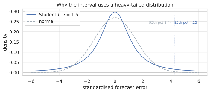
\(\nu = 1.5\) degrees of freedom is far below the Gaussian limit. The posterior variance formula would give a Gaussian band, and a Gaussian band on financial forecast errors is famously too narrow.

Show the code
from scipy import stats

grid = np.linspace(-6, 6, 600)
heavy, normal = stats.t(df=DSL_DEFAULTS.interval_df), stats.norm()
scale_t, scale_n = heavy.ppf(0.75), normal.ppf(0.75)

figure, axis = plt.subplots(figsize=(7.5, 3.4))
axis.plot(grid, heavy.pdf(grid * scale_t) * scale_t, color=pf.ACCENT,
          label=r"Student-$t$, $\nu$ = 1.5")
axis.plot(grid, normal.pdf(grid * scale_n) * scale_n, color=pf.GREY, ls="--",
          label="normal")
for distribution, scale, colour in ((heavy, scale_t, pf.ACCENT), (normal, scale_n, pf.GREY)):
    quantile = distribution.ppf(0.95) / scale
    axis.axvline(quantile, color=colour, lw=1, ls=":")
    axis.annotate(f"95th pct {quantile:.2f}", (quantile, 0.24), fontsize=8.5, color=colour)
axis.set(xlabel="standardised forecast error", ylabel="density")
axis.set_title("Why the interval uses a heavy-tailed distribution")
axis.legend()
figure.tight_layout()
Figure 2: A Student-t with 1.5 degrees of freedom against the normal, both scaled to unit interquartile range. A 90% band from the t is much wider in the tails.

Degrading gracefully, and refusing outright

The two are different, and the distinction is the interesting part of the port.

Show the code
short_record = subjects.assign(model_growth_error_variance=float("nan"))
degraded = method.fit(short_record).apply(short_record)
degraded_row = degraded.dropna(subset=["posterior_level"]).iloc[-1]

pd.DataFrame(
    [
        {
            "case": "full record",
            "weights": "prior, model, consensus",
            "published": True,
            "growth": f"{row.posterior_growth:+.4%}",
        },
        {
            "case": "model track record too short",
            "weights": "prior, consensus",
            "published": bool(degraded_row[pfc.ELIGIBLE_COLUMN]),
            "growth": f"{degraded_row.posterior_growth:+.4%}",
        },
    ]
)
case weights published growth
0 full record prior, model, consensus True +4.9481%
1 model track record too short prior, consensus True +4.3384%

A model whose record is too short to estimate a precision drops out of the blend and the subject is still published on prior and consensus. A model whose value is missing refuses the subject outright: there is nothing to weigh.

Show the code
missing_model = subjects.assign(model=float("nan"))
refused = method.fit(missing_model).apply(missing_model)
refused[[pfc.ELIGIBLE_COLUMN, pfc.ELIGIBILITY_REASON_COLUMN]].tail(1)
eligible eligibility_reason
8 False missing_prediction

Every refusal reason:

Show the code
pd.DataFrame(
    [{"reason": reason.value} for reason in PosteriorReason]
)
reason
0 publishable
1 missing_input
2 insufficient_history
3 no_consensus_precision
4 missing_prediction
5 nonfinite_result

Neither branch is a fallback in the forbidden sense — no unpublishable subject ever gets a substituted number. Both are declared method behaviour, taken from the reference, and both carry tests.

Settings are configuration, not a fitted set

Show the code
DSL_DEFAULTS.model_dump(mode="json")
{'minimum_observations': 3,
 'include_model': True,
 'consensus_stdev_variance_multiplier': 1.0,
 'consensus_count_exponent': None,
 'interval_width': 0.9,
 'interval_df': 1.5,
 'interval_loc': 0.5,
 'interval_scale': 2.75,
 'dispersion_weighted': False,
 'version': 'dsl-defaults'}

Note what is missing: a fitted_through date. The anchored estimate’s parameters were fitted by regression on a training sample, so they carry the date their training data ended. These are the production DSL’s defaults — chosen, not estimated — so there is nothing to date. They still carry a version, because a published number depends on them.

Show the code
patient = BayesianSettings(
    **{**DSL_DEFAULTS.model_dump(), "minimum_observations": 6, "version": "patient-demo"}
)
pd.DataFrame(
    [
        {
            "settings": settings.version,
            "minimum_observations": settings.minimum_observations,
            "declared minimum_history": BayesianPosterior(
                forecast_source="model", settings=settings
            ).requirements.minimum_history,
        }
        for settings in (DSL_DEFAULTS, patient)
    ]
)
settings minimum_observations declared minimum_history
0 dsl-defaults 3 3
1 patient-demo 6 6

The declared requirement follows the setting, so a pipeline assembled with patient settings advertises what it actually needs.

How the two methods relate

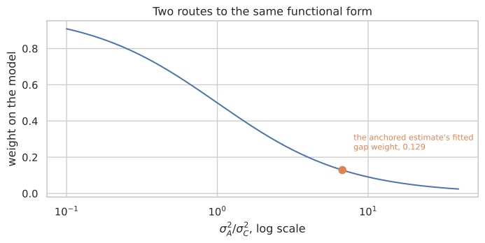
Drop the prior from the blend and the two-source case rearranges into exactly the anchored form:

\[ \hat\theta = x_C + \underbrace{\frac{\sigma_C^2}{\sigma_A^2 + \sigma_C^2}}_{w_A}\,(x_A - x_C) \]

Compare with the anchored level, \(\hat y = c + b_g (m - c)\). The two are the same estimator with

\[ b_g \longleftrightarrow w_A = \frac{1}{1 + \sigma_A^2/\sigma_C^2} \]

Same functional form, different estimand. The regression estimates that ratio from the joint distribution of gap and surprise, across companies. The Bayesian computes it from each source’s own error history, per company.

Show the code
ratio = np.logspace(-1, 1.6, 400)
curve = pd.DataFrame({"ratio": ratio, "weight": 1 / (1 + ratio)})

figure, axis = plt.subplots(figsize=(7.5, 3.8))
sns.lineplot(data=curve, x="ratio", y="weight", ax=axis, color=pf.ACCENT)
fitted = pfc.STUDY_2025_01.gap_weight
axis.scatter([(1 - fitted) / fitted], [fitted], s=60, color=pf.WARM, zorder=3)
axis.annotate(
    f"the anchored estimate's fitted\ngap weight, {fitted}",
    ((1 - fitted) / fitted, fitted), xytext=(12, 22), textcoords="offset points",
    fontsize=8.5, color=pf.WARM,
)
axis.set_xscale("log")
axis.set(xlabel=r"$\sigma_A^2/\sigma_C^2$, log scale", ylabel="weight on the model")
axis.set_title("Two routes to the same functional form")
figure.tight_layout()
Figure 3: The weight on the model as a function of the error-variance ratio. The anchored estimate’s fitted gap weight of 0.129 is one point on this curve.

A measured median error of 2.99% for the model against 1.54% for consensus implies a weight near 0.21 if the two errors were independent. The regression says 0.129. The wedge between them is error correlation: both track the same company, so their errors move together, and a naive precision weighting over-weights the model. The independent variant is the DSL’s default anyway, because covariance estimates are materially less stable than scalar variances when two sources are strongly collinear.

What to take away

  • Precisions add, weights are precision shares. Both facts fall out of the algebra, and both are asserted per subject in the tests.
  • Growth space is what makes a variance meaningful. Levels are non-stationary.
  • Point-in-time is harder here than for the anchored estimate. Every error in the record has to be measured against what a source said before the actual landed.
  • Degrading and refusing are different. A short record drops a source; a missing value refuses the subject.
  • Settings carry a version but no fitted-through date, because nothing in them was fitted.