flowchart LR
    A[Existing model<br>produces forecast] --> B[Post-processing<br>read inputs as of now]
    C[Consensus and<br>realised history] --> B
    B --> D[Publish adjusted estimate<br>or record refusal]
    D --> E[Outcome arrives later]
    E --> F[Compare errors<br>before changing policy]
Can post-processing improve a forecast?
A practical workflow, followed by a six-period Apple comparison
An existing forecasting system stays in place. It produces a forecast; this notebook adds a post-processing step before publication, then measures whether that step improves accuracy when the outcome arrives.
- Normal use: Supply the model forecast, a matching consensus, and the timestamp at which each became available. Bayesian combination also needs historical forecasts and actuals.
- Possible benefit: Reduce a noisy model’s influence using consensus and its historical reliability, or apply a previously calibrated consensus-relative rule.
- Possible cost: Pull a good forecast toward a worse reference. Adjustment cannot create information that the inputs do not contain.
- Decision: Compare against both the original model and consensus on the same future outcomes, while retaining refusal counts.
This notebook loads the same real ADC export as the detailed model walkthrough. It first demonstrates a current publication call, then replays six historical forecasting dates with illustrative plots. The historical model is reconstructed: this is a conditional comparison within one export vintage, not a verified live out-of-sample trial.
1. Where it fits in the normal workflow
- Keep the model: The library does not retrain it or read its raw predictors.
- Match the target: Model, consensus, and actual must describe the same company, fiscal period, quantity, and units.
- Preserve observations: Keep forecast revisions and actual availability timestamps. Overwriting history prevents a defensible evaluation.
- Choose one method: Anchoring and the Bayesian posterior are alternatives. Applying one after the other is not the workflow demonstrated here.
- Separate learning and publication: Anchoring uses frozen coefficients. Bayesian moments come from outcomes already known at each reading moment.
2. Load a forecast and its history
Run just install, select .venv/bin/python, and run this notebook from docs/. POSTFORECAST_EXPORT can point at another export with universe.parquet and signals/. Missing exports stop execution; no synthetic substitute is used.
The default is the ADC Core export used in the companion walkthrough. Its file hashes and model IDs are displayed there. The source’s date-only availability values are interpreted as UTC midnight, not as verified intraday delivery times.
import os
from pathlib import Path

import matplotlib.pyplot as plt
import numpy as np
import pandas as pd
import tutorial_support as examples
from IPython.display import display as show

import postforecast as pf

examples.set_style()
export_root = Path(
    os.environ.get(
        "POSTFORECAST_EXPORT",
        "~/repos/adc-models/data/customers-371/line-items/190/2026-09-20",
    )
).expanduser()
ticker = "AAPL"
universe = pd.read_parquet(export_root / "universe.parquet")
company = universe.loc[universe.ticker.eq(ticker) & universe.country.eq("US")].squeeze()
frames = []
for signal, source in {
    "model_prediction": "live_model",
    "model_pit_backtest": "historical_model",
    "consensus": "consensus",
    "actual": "actual",
}.items():
    path = export_root / "signals" / f"signal_type={signal}" / "data.parquet"
    frames.append(
        pd.read_parquet(path, filters=[("entity_id", "==", company.entity_id)]).assign(
            source=source
        )
    )
raw = pd.concat(frames, ignore_index=True)
panel = pf.validate_estimates(
    raw.rename(
        columns={
            "entity_id": "entity",
            "period_end_date": "period",
        }
    ).assign(
        target="revenue",
        period_end=pd.to_datetime(raw.period_end_date, utc=True),
        known_at=pd.to_datetime(raw.known_at, utc=True),
    )
)
keys = ["entity", "period", "target", "period_end"]
examples.format_dates(
    panel.groupby("source", as_index=False).agg(
        rows=("value", "size"),
        latest_available=("known_at", "max"),
    )
)| source | rows | latest_available | |
|---|---|---|---|
| 0 | actual | 17104 | 2026-09-13 |
| 1 | consensus | 10014 | 2026-09-16 |
| 2 | historical_model | 339 | 2026-09-07 |
| 3 | live_model | 22 | 2026-09-20 |
3. Publish after the existing model has run
Use an explicit reading time and target period. These calls belong in the application after it obtains the model’s prediction and before it publishes a number.
- Anchoring:
publish_anchoredreturns the adjusted level, expected surprise, and publication verdict. The shipped Core coefficients illustrate a previously fitted policy; deploying them for a changed model vintage requires validation. - Bayesian:
bayesian_kpi_predictionsreads live predictions and learns precisions from the separate historical-model source. Minimum history and uncertainty settings are explicit in its settings object. - Caller responsibility: The anchored method checks source ages. The Bayesian API does not inherit those age limits; the application must choose its own freshness policy before using it in production.
parameters = pf.CORE_2025_01
settings = pf.BayesianPredictionSettings(
    version="forecast-improvement-example-v1",
    series="predictions",
    minimum_observations=3,
    values=("prediction", "prediction-lower", "prediction-upper"),
)
publication_time = pd.Timestamp("2026-09-22", tz="UTC")
publication_period = "2026-09-26"
requested = panel.loc[panel.period.eq(publication_period), keys].drop_duplicates()
anchored_now = pf.publish_anchored(
    panel,
    publication_time,
    forecast_source="live_model",
    parameters=parameters,
    subjects=requested,
    fields=("anchored_level", "expected_surprise"),
)
bayesian_now = pf.bayesian_kpi_predictions(
    panel,
    publication_time,
    forecast_source="live_model",
    backtest_source="historical_model",
    settings=settings,
)
show(anchored_now[["period", "anchored_level", "eligible", "eligibility_reason"]])
show(
    bayesian_now.loc[
        bayesian_now.period.eq(publication_period),
        ["period", "prediction", "prediction-lower", "prediction-upper", "eligible"],
    ]
)| period | anchored_level | eligible | eligibility_reason | |
|---|---|---|---|---|
| 0 | 2026-09-26 | 1.154643e+11 | True | publishable |
| period | prediction | prediction-lower | prediction-upper | eligible | |
|---|---|---|---|---|---|
| 0 | 2026-09-26 | 1.136502e+11 | 7.209368e+10 | 1.594956e+11 | True |
Do not publish merely because a cell contains a number. Check eligible, retain eligibility_reason, and store the full settings or parameter payload. Preserve the raw model and consensus beside the adjusted output so future accuracy can be evaluated. A current estimate has no known error yet.
4. Define the comparison before measuring results
The historical replay uses a fixed schedule, rather than selecting whichever forecast date looks best after seeing the outcome.
- Company: Apple, the same company as the current-publication example.
- Target window: Fiscal period ends from January 2025 through June 2026.
- Forecast date: Fourteen calendar days after each fiscal period end. This is an explicit tutorial policy, not a recommended universal horizon.
- Training boundary: Each calculation receives only observations strictly before its forecast date. Each target’s outcome must still be unknown then.
- Anchoring coefficients: Frozen through 2024-12-31; not refitted on the evaluation periods. No coefficient is selected using the results below.
- Bayesian history: Expands as earlier outcomes become available. Every historical replay uses the reconstructed model as its forecast source.
- Scoring actual: The first actual present in this export for each period. This may differ from the original release if the export backfills history.
- Comparison sample: Only periods with finite outputs from all four methods enter the paired error comparison. Coverage and refusals are shown first.
No market returns, trading costs, or stock-price reactions enter this accuracy exercise. The calculation belongs in the notebook; evaluation is not added to the postforecast library.
actuals = (
    panel.loc[panel.source.eq("actual")]
    .sort_values("known_at")
    .drop_duplicates(["entity", "period", "target"])
    .sort_values("period_end")
)
targets = actuals.loc[
    actuals.period_end.between(
        pd.Timestamp("2025-01-01", tz="UTC"),
        pd.Timestamp("2026-06-30", tz="UTC"),
    )
].copy()
targets["forecast_date"] = targets.period_end + pd.Timedelta(days=14)
np.testing.assert_equal(
    bool(targets.forecast_date.lt(targets.known_at).all()), desired=True
)
np.testing.assert_equal(
    bool(
        targets.forecast_date.gt(
            pd.Timestamp(parameters.fitted_through, tz="UTC")
        ).all()
    ),
    desired=True,
)
examples.format_dates(
    targets[["period", "forecast_date", "known_at"]].rename(
        columns={"known_at": "outcome_available"},
    )
)| period | forecast_date | outcome_available | |
|---|---|---|---|
| 24236 | 2025-03-29 | 2025-04-12 | 2025-05-01 |
| 24452 | 2025-06-28 | 2025-07-12 | 2025-07-31 |
| 24690 | 2025-09-27 | 2025-10-11 | 2025-10-30 |
| 24946 | 2025-12-27 | 2026-01-10 | 2026-01-29 |
| 25189 | 2026-03-28 | 2026-04-11 | 2026-04-30 |
| 25436 | 2026-06-27 | 2026-07-11 | 2026-07-30 |
5. Replay the same post-processing step
The loop reads the target’s actual only when recording the result for scoring. That actual never enters the panel supplied to either method. The historical model is used here because live predictions in this export cover current periods rather than the whole evaluation window.
records = []
for target in targets.itertuples():
    cutoff = target.forecast_date
    known = panel.loc[panel.known_at.lt(cutoff)]
    requested = panel.loc[panel.period.eq(target.period), keys].drop_duplicates()
    prepared = pf.prepare_anchored_subjects(
        known,
        cutoff,
        forecast_source="historical_model",
        subjects=requested,
    )
    anchored = (
        pf.AnchoredEstimate(
            forecast_source="forecast",
            parameters=parameters,
        )
        .fit(prepared)
        .apply(prepared)
        .iloc[0]
    )
    posterior_rows = pf.bayesian_kpi_predictions(
        known,
        cutoff,
        forecast_source="historical_model",
        settings=settings,
    )
    posterior = posterior_rows.set_index("period").reindex([target.period]).iloc[0]
    records.append(
        {
            "period": target.period,
            "forecast_date": cutoff,
            "actual_known_at": target.known_at,
            "Actual": target.value,
            "Raw model": anchored.forecast,
            "Consensus": anchored.consensus,
            "Anchored": anchored.anchored_level,
            "Bayesian": posterior["prediction"],
            "anchored_eligible": anchored.eligible,
            "anchored_reason": anchored.eligibility_reason,
            "bayesian_eligible": posterior.eligible,
            "bayesian_reason": posterior.eligibility_reason,
        }
    )
results = pd.DataFrame(records).set_index("period")
methods = ["Raw model", "Consensus", "Anchored", "Bayesian"]
finite = np.isfinite(results[methods]).all(axis=1)
paired = results.loc[
    finite
    & results.anchored_eligible.eq(other=True)
    & results.bayesian_eligible.eq(other=True)
]
show(
    results[
        ["anchored_eligible", "anchored_reason", "bayesian_eligible", "bayesian_reason"]
    ]
)
print(f"Paired comparison: {len(paired)} of {len(results)} target periods.")
if paired.empty:
    message = "No common eligible periods. Inspect coverage before comparing accuracy."
raise ValueError(message)| anchored_eligible | anchored_reason | bayesian_eligible | bayesian_reason | |
|---|---|---|---|---|
| period | ||||
| 2025-03-29 | True | publishable | True | eligible |
| 2025-06-28 | True | publishable | True | eligible |
| 2025-09-27 | True | publishable | True | eligible |
| 2025-12-27 | True | publishable | True | eligible |
| 2026-03-28 | True | publishable | True | eligible |
| 2026-06-27 | True | publishable | True | eligible |
Paired comparison: 6 of 6 target periods.6. See how adjustment changes one forecast
The first evaluation period is selected by date, before looking at its error. The later actual is drawn only as an evaluation reference. In a real forecast run, that vertical line would not yet exist.
Read the arrows: Moving toward consensus helps if the raw model’s deviation is mostly error. It hurts if that deviation contains information that consensus misses. Anchoring can also move beyond consensus through its intercept and revision contribution.
first = paired.iloc[0]
fig, ax = plt.subplots(figsize=(10, 4))
for position, method in enumerate(methods):
    value = first[method] / 1e9
    ax.scatter(value, position, s=70, zorder=3)
    if method in {"Anchored", "Bayesian"}:
        ax.annotate(
            "",
            xy=(value, position),
            xytext=(first["Raw model"] / 1e9, position),
            arrowprops={"arrowstyle": "->", "color": examples.ACCENT, "lw": 2},
        )
ax.axvline(first.Actual / 1e9, color="black", linestyle="--", label="Later actual")
ax.set(
    yticks=range(len(methods)),
    yticklabels=methods,
    xlabel="Revenue (export units, billions)",
    title=f"{ticker}: {paired.index[0]}",
)
ax.legend()
plt.show()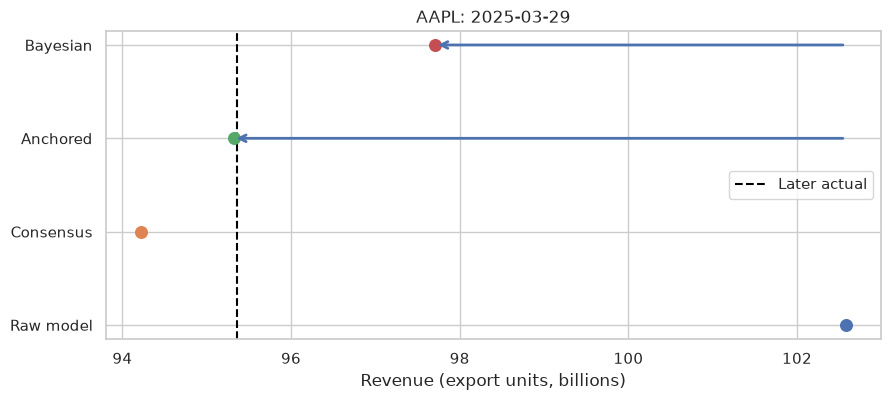
7. Measure improvement over the whole selected window
For forecast \(F\) and actual \(A\), percentage error is \(100(F-A)/A\). The outcome denominators here are positive revenue values.
- Mean absolute percentage error (MAPE): Average absolute error as a percentage of actual revenue; lower is better.
- Mean signed percentage error: Average bias; positive means overprediction. Errors can cancel, so a small bias alone does not imply accuracy.
- Improvement versus raw: Raw model MAPE minus adjusted MAPE, in percentage points. A positive value means lower average error in this paired sample.
- Consensus baseline: An adjusted forecast should also be judged against using consensus alone. Beating a weak raw model is an incomplete result.
np.testing.assert_equal(bool(paired.Actual.gt(0).all()), desired=True)
errors = paired[methods].sub(paired.Actual, axis=0).div(paired.Actual, axis=0) * 100
absolute_errors = errors.abs()
summary = pd.DataFrame(
    {
        "Periods": len(paired),
        "MAPE (%)": absolute_errors.mean(),
        "Mean signed error (%)": errors.mean(),
    }
)
summary["Improvement vs raw (pp)"] = (
    summary.loc["Raw model", "MAPE (%)"] - summary["MAPE (%)"]
)
summary.round(3)| Periods | MAPE (%) | Mean signed error (%) | Improvement vs raw (pp) | |
|---|---|---|---|---|
| Raw model | 6 | 5.420 | -1.617 | 0.000 |
| Consensus | 6 | 2.486 | -2.486 | 2.934 |
| Anchored | 6 | 1.520 | -1.520 | 3.900 |
| Bayesian | 6 | 2.763 | -1.941 | 2.657 |
fig, ax = plt.subplots(figsize=(9, 4))
values = summary["MAPE (%)"]
bars = ax.bar(
    values.index,
    values,
    color=[examples.MUTED, examples.WARM, examples.ACCENT, "#55a868"],
)
ax.bar_label(bars, fmt="%.2f%%", padding=4)
ax.set(ylabel="Mean absolute percentage error (%)", ylim=(0, values.max() * 1.2))
plt.show()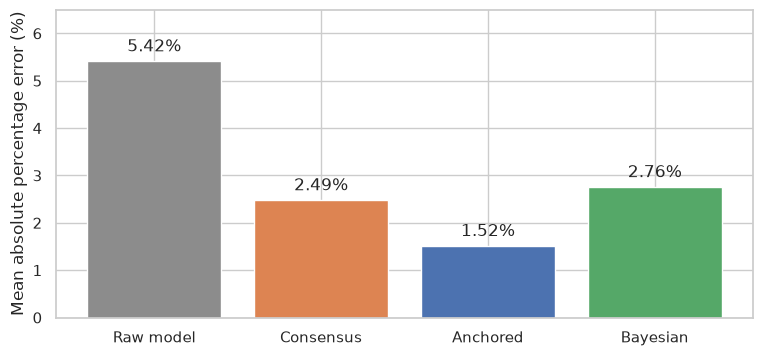
8. Find the periods where it hurts
An average can hide a bad individual forecast. This chart shows the change in absolute percentage error for each target period. Positive bars mean improvement; negative bars mean the adjustment was worse than the raw model.
A method that helps on average still needs monitoring. The six observations here are too few to establish stable performance across companies or regimes.
improvement = absolute_errors[["Consensus", "Anchored", "Bayesian"]].rsub(
    absolute_errors["Raw model"],
    axis=0,
)
fig, ax = plt.subplots(figsize=(11, 4.5))
improvement.plot.bar(ax=ax, color=[examples.WARM, examples.ACCENT, "#55a868"])
ax.axhline(0, color="black", linewidth=1)
ax.set(
    xlabel="Fiscal period end", ylabel="Reduction in absolute error (percentage points)"
)
ax.tick_params(axis="x", rotation=30)
ax.legend(title="")
fig.tight_layout()
plt.show()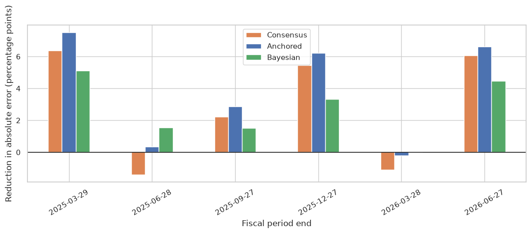
worse = improvement.lt(0).sum().rename("Periods worse than raw")
show(worse.to_frame())
print(f"Raw model MAPE: {summary.loc['Raw model', 'MAPE (%)']:.2f}%")
print(f"Anchored MAPE: {summary.loc['Anchored', 'MAPE (%)']:.2f}%")
print(f"Bayesian MAPE: {summary.loc['Bayesian', 'MAPE (%)']:.2f}%")
print(f"Consensus MAPE: {summary.loc['Consensus', 'MAPE (%)']:.2f}%")| Periods worse than raw | |
|---|---|
| Consensus | 2 |
| Anchored | 1 |
| Bayesian | 1 |
Raw model MAPE: 5.42%
Anchored MAPE: 1.52%
Bayesian MAPE: 2.76%
Consensus MAPE: 2.49%
For the saved default export, both adjusted methods beat the raw model on average, while the Bayesian result has more average error than consensus alone. Both adjustments also hurt on at least one individual period. The tables and plots above are the computed evidence; changing the input can change that conclusion.
9. Check the time boundary
The first target’s outcome and all later observations are removed in the replay. The library’s own as-of read should give exactly the same posterior when given the complete panel instead. This check would fail if future rows changed that calculation. It does not test whether the upstream model selection was historically available; that remains an export-provenance limitation.
first_target = targets.iloc[0]
full_read = pf.bayesian_kpi_predictions(
    panel,
    first_target.forecast_date,
    forecast_source="historical_model",
    settings=settings,
)
limited_read = pf.bayesian_kpi_predictions(
    panel.loc[panel.known_at.lt(first_target.forecast_date)],
    first_target.forecast_date,
    forecast_source="historical_model",
    settings=settings,
)
pd.testing.assert_frame_equal(full_read, limited_read)
np.testing.assert_allclose(
    improvement["Anchored"].mean(),
    summary.loc["Anchored", "Improvement vs raw (pp)"],
)
print(
    "Checks passed: outcomes follow forecasts; future rows do not change the read; error attribution agrees."
)
Checks passed: outcomes follow forecasts; future rows do not change the read; error attribution agrees.10. Turn the exercise into a normal operating process
- Capture: Append each newly produced model forecast and the matching consensus with their true availability timestamps.
- Post-process: At a scheduled reading moment, run the chosen method and retain its verdict, parameter payload, input snapshot, and software revision.
- Publish: Release eligible results under a stable policy. Preserve refusals and use any alternative publication policy explicitly, not as a silent fallback.
- Score later: Append the first reported outcome when available, then compare raw, adjusted, and consensus errors on matching targets and horizons.
- Monitor coverage: Track failures and source freshness alongside accuracy. Lower error obtained only by declining difficult forecasts is not a like-for-like win.
- Recalibrate deliberately: Fit new coefficients or choose settings on a training/validation window. Freeze them, version them, and assess later untouched observations before replacing the published policy.
What would justify adoption? Consistent improvements on untouched future observations, useful coverage, and acceptable errors in the cases that matter to the application. Include consensus as a baseline and evaluate interval coverage separately if publishing uncertainty bands.
What this example establishes: A working integration and a reproducible within-export comparison. It cannot establish live predictive improvement because the historical model vintage was reconstructed and the sample is small.
Continue with the detailed real-model calculations, anchoring methodology, or Bayesian posterior. The terminology introduction defines the data and method terms.