A real model, two published estimates

Apple revenue: read the export, anchor the inputs, and explain the posterior

Start with the introduction for terminology. This notebook loads real ADC model data and follows one fiscal period through both methods. Each figure comes from the loaded data and the installed library.

1. Choose the export and the question

Run just install in the postforecast checkout and select .venv/bin/python as the kernel. Run the notebook from docs/, alongside pf.py. The export files stay in the source repository; no vendor client or credential is needed to read an already downloaded export.

  • Default export: ~/repos/adc-models/data/customers-371/line-items/190/2026-09-20.
  • Alternate location: Set POSTFORECAST_EXPORT to a directory containing universe.parquet and signals/. The buy-side study’s BSC_SIGNALS layout has the same structure; point this variable at that directory to use it.
  • Pinned selection: The directory, entity, target period, and as-of date are explicit below. Changing the export requires reviewing model provenance and the anchoring coefficient choice, not merely rerunning the cells.
  • Missing data: Execution stops with the missing path; synthetic data is never substituted. Existing rendered outputs remain readable without local exports.
import hashlib
import os
from pathlib import Path

import matplotlib.pyplot as plt
import numpy as np
import pandas as pd
import tutorial_support as examples
from IPython.display import display as show

import postforecast as pf

examples.set_style()
export_root = Path(
    os.environ.get(
        "POSTFORECAST_EXPORT",
        "~/repos/adc-models/data/customers-371/line-items/190/2026-09-20",
    )
).expanduser()
ticker = "AAPL"
period = "2026-09-26"
as_of = pd.Timestamp("2026-09-22", tz="UTC")
parameters = pf.CORE_2025_01

universe = pd.read_parquet(export_root / "universe.parquet")
company = universe.loc[universe.ticker.eq(ticker) & universe.country.eq("US")].squeeze()
entity = company.entity_id
pd.DataFrame(
    {
        "setting": [
            "company",
            "entity",
            "period end",
            "as of (exclusive UTC)",
            "export directory",
            "coefficient version",
        ],
        "value": [
            company.company_name,
            entity,
            period,
            as_of.strftime("%Y-%m-%d"),
            export_root.name,
            parameters.version,
        ],
    }
)
setting value
0 company Apple, Inc.
1 entity graph:entity::company::F_000C7F-E
2 period end 2026-09-26
3 as of (exclusive UTC) 2026-09-22
4 export directory 2026-09-20
5 coefficient version core-2025-01

2. Load observations, retaining their provenance

  • Live model: model_prediction supplies the current forecast.
  • Historical model: model_pit_backtest supplies reconstructed historical forecasts. Keeping it separate prevents silently splicing different source roles.
  • Consensus: The analyst reference level for the same entity and period.
  • Actual: The outcome observations available in this export, including revisions.
  • Memory: Parquet filters select one entity before loading its rows into pandas.
  • Dates: These files encode availability as dates. Parsing as UTC midnight preserves that date convention; it does not establish intraday delivery timing.

The hashes identify the exact files read. The directory’s date is a label, not a substitute for checking the timestamps inside those files.

source_names = {
    "model_prediction": "model",
    "model_pit_backtest": "model_history",
    "consensus": "consensus",
    "actual": "actual",
}
frames = []
provenance = []
for signal, source in source_names.items():
    path = export_root / "signals" / f"signal_type={signal}" / "data.parquet"
    observations = pd.read_parquet(path, filters=[("entity_id", "==", entity)])
    with path.open("rb") as stream:
        digest = hashlib.file_digest(stream, "sha256").hexdigest()
    provenance.append(
        {"source": source, "rows loaded": len(observations), "sha256": digest}
    )
    frames.append(observations.assign(source=source))
raw = pd.concat(frames, ignore_index=True)
show(pd.DataFrame(provenance))
show(
    raw.loc[
        raw.source.isin(["model", "model_history"]), ["source", "model_id"]
    ].drop_duplicates()
)
source rows loaded sha256
0 model 22 9b7705d30e4d8aedff1a698ead3b8fd93325db3db8c401...
1 model_history 339 429e597b850ee659dd9004360a010a57dcb7eeb57d9d3c...
2 consensus 10014 ca282ca6e97febae3794574d0d4e341747a33bdb8fbc35...
3 actual 17104 4f9d8c87761abd96a5c86049c94e9ae4c78c030cce7cdd...
source model_id
0 model 303124
22 model_history 303124
ImportantA historical cutoff is not a historical model snapshot

The ADC repository’s docs/export-vintage-analysis.md documents that later exports can contain changed historical forecasts after model replacement. model_pit_backtest reconstructs history using the selected model and stored input versions. Its known_at column alone does not prove that model selection, tuning, or vendor data existed as shown on the historical date.

The calculations below respect the timestamps supplied. They demonstrate the methodology on this export, without claiming a tradable historical record.

3. Form a tidy estimate panel

One row means one source’s value for one subject at one availability time. The source’s fiscal period-end date becomes the opaque period label, avoiding an incorrect assumption about calendar quarters. Monetary values retain their export units throughout calculation; charts scale them to billions.

Extra provenance columns such as model_id remain attached. The panel validator rejects duplicate observation keys instead of averaging conflicting records.

panel = raw.rename(columns={"entity_id": "entity", "period_end_date": "period"}).assign(
    target="revenue",
    period_end=pd.to_datetime(raw.period_end_date, utc=True),
    known_at=pd.to_datetime(raw.known_at, utc=True),
)
panel = pf.validate_estimates(panel)
coverage = panel.groupby("source", as_index=False).agg(
    observations=("value", "size"),
    periods=("period", "nunique"),
    first_available=("known_at", "min"),
    last_available=("known_at", "max"),
)
show(examples.format_dates(coverage))
show(
    examples.format_dates(
        panel.loc[
            panel.period.eq(period),
            ["entity", "period", "target", "source", "known_at", "value"],
        ].tail(8)
    )
)
source observations periods first_available last_available
0 actual 17104 75 2008-01-22 2026-09-13
1 consensus 10014 66 2012-10-02 2026-09-16
2 model 22 2 2026-09-10 2026-09-20
3 model_history 339 15 2023-06-05 2026-09-07
entity period target source known_at value
25957 graph:entity::company::F_000C7F-E 2026-09-26 revenue model_history 2026-07-20 1.118946e+11
25958 graph:entity::company::F_000C7F-E 2026-09-26 revenue model_history 2026-07-27 1.094226e+11
25959 graph:entity::company::F_000C7F-E 2026-09-26 revenue model_history 2026-08-03 1.163147e+11
25960 graph:entity::company::F_000C7F-E 2026-09-26 revenue model_history 2026-08-10 1.152416e+11
25961 graph:entity::company::F_000C7F-E 2026-09-26 revenue model_history 2026-08-17 1.140443e+11
25962 graph:entity::company::F_000C7F-E 2026-09-26 revenue model_history 2026-08-24 1.140732e+11
25963 graph:entity::company::F_000C7F-E 2026-09-26 revenue model_history 2026-08-31 1.145663e+11
25964 graph:entity::company::F_000C7F-E 2026-09-26 revenue model_history 2026-09-07 1.142456e+11

4. Freeze the reading moment

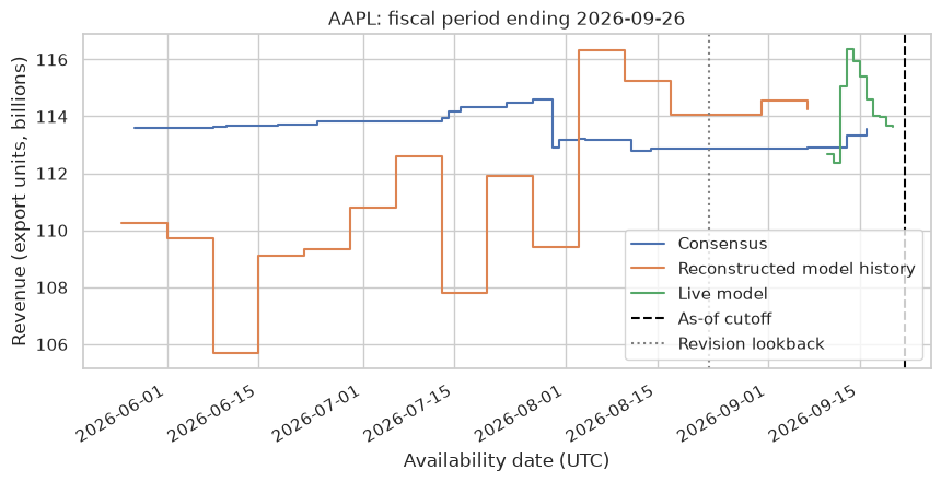
The first chart follows one target period through availability time. It is not a chart of revenue across quarters. A source can revise the same period many times; only its latest observation strictly before the cutoff is read.

The 30-day marker is the earlier consensus reading used for the revision. A line ending before the cutoff means the latest available observation is older than the reading moment; the library does not invent an update.

subject_panel = panel.loc[panel.period.eq(period)]
fig, ax = plt.subplots(figsize=(10, 4.5))
for source, label in [
    ("consensus", "Consensus"),
    ("model_history", "Reconstructed model history"),
    ("model", "Live model"),
]:
    observations = subject_panel.loc[
        subject_panel.source.eq(source)
        & subject_panel.known_at.ge(as_of - pd.Timedelta(days=120))
    ].sort_values("known_at")
    ax.step(observations.known_at, observations.value / 1e9, where="post", label=label)
ax.axvline(as_of, color="black", linestyle="--", label="As-of cutoff")
ax.axvline(
    as_of - pd.Timedelta(days=30),
    color="gray",
    linestyle=":",
    label="Revision lookback",
)
ax.set(
    xlabel="Availability date (UTC)",
    ylabel="Revenue (export units, billions)",
    title=f"{ticker}: fiscal period ending {period}",
)
ax.legend(loc="best")
fig.autofmt_xdate()
plt.show()
Model and consensus across availability dates with cutoff markers.
Figure 1: One target period, two reading moments.
snapshot = pf.latest_before(subject_panel, as_of)
show(examples.format_dates(snapshot[["source", "known_at", "value"]]))
subjects = pf.prepare_anchored_subjects(
    panel,
    as_of,
    forecast_source="model",
    subjects=subject_panel[
        ["entity", "period", "target", "period_end"]
    ].drop_duplicates(),
)
show(
    examples.format_dates(
        subjects[
            [
                "period",
                "forecast",
                "forecast_known_at",
                "forecast_age",
                "consensus",
                "consensus_known_at",
                "consensus_age",
                "consensus_revision",
            ]
        ]
    )
)
source known_at value
0 consensus 2026-09-16 1.135637e+11
1 model 2026-09-20 1.136439e+11
2 model_history 2026-09-07 1.142456e+11
period forecast forecast_known_at forecast_age consensus consensus_known_at consensus_age consensus_revision
0 2026-09-26 1.136439e+11 2026-09-20 2 days 1.135637e+11 2026-09-16 6 days 0.00632

5. Explain the consensus-anchored estimate

Let \(M\) be the model, \(C\) consensus, and \(C_{-30}\) the earlier consensus reading.

\[ \text{gap}=M/C-1,\qquad r=C/C_{-30}-1 \]

\[ \widehat{s}=a+b\,\text{gap}+c\,r,\qquad \widehat{Y}_{\mathrm{anchored}}=C(1+\widehat{s}) \]

  • Customary beat: \(a\), the fitted intercept.
  • Model contribution: \(b\) times the current gap.
  • Revision contribution: \(c\) times the consensus revision.
  • Frozen coefficients: CORE_2025_01 is the shipped Core example, trained through 2024-12-31. Applying it to this later export demonstrates the arithmetic; it does not validate those coefficients for the export’s changed model vintage.
  • Missing earlier consensus: The method explicitly drops the revision term when no revision can be measured. Other missing required inputs can cause refusal.

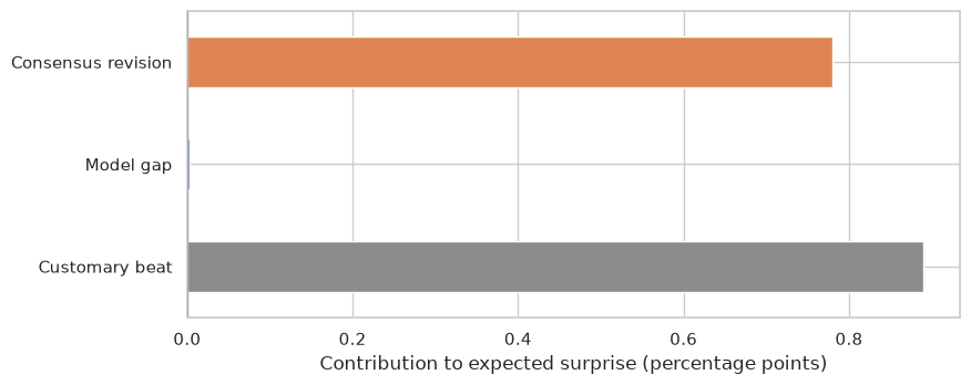
The contribution chart measures percentage points of expected surprise, not revenue dollars. The contributions must sum to the published surprise.

anchoring = pf.AnchoredEstimate(forecast_source="forecast", parameters=parameters).fit(
    subjects
)
anchored = anchoring.apply(subjects)
show(
    anchored[
        [
            "period",
            "anchored_level",
            "expected_surprise",
            "eligible",
            "eligibility_reason",
            "parameters_version",
        ]
    ]
)
contributions = anchored.iloc[0][
    ["contribution_customary_beat", "contribution_gap", "contribution_revision"]
].astype(float)
contributions.index = ["Customary beat", "Model gap", "Consensus revision"]
contributions.mul(100).to_frame("Contribution (percentage points)")
period anchored_level expected_surprise eligible eligibility_reason parameters_version
0 2026-09-26 1.154643e+11 0.016736 True publishable core-2025-01
Contribution (percentage points)
Customary beat 0.890000
Model gap 0.003119
Consensus revision 0.780445
fig, ax = plt.subplots(figsize=(9, 3.6))
contributions.mul(100).plot.barh(
    ax=ax, color=[examples.MUTED, examples.ACCENT, examples.WARM]
)
ax.axvline(0, color="black", linewidth=0.8)
ax.set(xlabel="Contribution to expected surprise (percentage points)", ylabel="")
plt.show()
Bars for customary beat, model gap, and consensus revision.
Figure 2: Three contributions sum to expected surprise.

6. Build the independent Bayesian posterior

The Bayesian route learns uncertainty from the company’s realised history. Historical model and consensus readings are selected strictly before each period’s first actual timestamp present in the export. Forward moments use only actuals available before the outer as_of moment.

  • First observed actual: This API retains the first actual in the export for each period. If earlier original reports are absent, that is a provenance gap; later data cannot repair it by relabelling a timestamp.
  • Prior growth: Mean and sample variance of sequential realised growth.
  • Model uncertainty: Mean squared historical model growth error.
  • Consensus uncertainty: Mean squared historical consensus growth error.
  • Separate histories: backtest_source="model_history" learns from reconstructed history, while forecast_source="model" supplies the current reading.
  • Basic configuration: Bias correction and analyst-dispersion weighting stay off so every weight is explained by the historical errors. The independent reference covers those extensions.

For precisions \(\tau_i\) and corresponding growth readings \(g_i\):

\[ w_i=\frac{\tau_i}{\tau_0+\tau_M+\tau_C},\qquad \mu_{\mathrm{post}}=w_0\mu_0+w_Mg_M+w_Cg_C. \]

The same previous actual \(A_{\mathrm{prev}}\) converts every reading to growth: \(g_M=M/A_{\mathrm{prev}}-1\) and \(g_C=C/A_{\mathrm{prev}}-1\). The posterior level is \(A_{\mathrm{prev}}(1+\mu_{\mathrm{post}})\).

settings = pf.BayesianPredictionSettings(
    version="adc-walkthrough-independent-v1",
    method="independent",
    series="predictions",
    values=(
        "prediction",
        "prediction-lower",
        "prediction-upper",
        "prior-mean",
        "model-growth",
        "consensus-growth",
        "posterior-growth",
        "prior-precision",
        "model-precision",
        "consensus-precision",
        "prior-weight",
        "model-weight",
        "consensus-weight",
    ),
)
posteriors = pf.bayesian_kpi_predictions(
    panel,
    as_of,
    forecast_source="model",
    backtest_source="model_history",
    settings=settings,
)
posterior = posteriors.loc[posteriors.period.eq(period)].iloc[0]
ingredients = pd.DataFrame(
    {
        "Ingredient": ["Prior", "Model", "Consensus"],
        "Growth": [
            posterior["prior-mean"],
            posterior["model-growth"],
            posterior["consensus-growth"],
        ],
        "Precision": [
            posterior[f"{name}-precision"] for name in ["prior", "model", "consensus"]
        ],
        "Weight": [
            posterior[f"{name}-weight"] for name in ["prior", "model", "consensus"]
        ],
    }
)
ingredients["Weighted growth"] = ingredients.Growth * ingredients.Weight
show(ingredients)
show(
    posteriors.loc[
        posteriors.period.eq(period),
        ["period", "prediction", "prediction-lower", "prediction-upper", "eligible"],
    ]
)
Ingredient Growth Precision Weight Weighted growth
0 Prior 0.069290 11.997931 0.018435 0.001277
1 Model 0.038631 187.554326 0.288174 0.011132
2 Consensus 0.037899 451.284838 0.693391 0.026279
period prediction prediction-lower prediction-upper eligible
0 2026-09-26 1.136502e+11 7.209368e+10 1.594956e+11 True
fig, axes = plt.subplots(1, 2, figsize=(11, 4))
colors = [examples.MUTED, examples.ACCENT, examples.WARM]
axes[0].bar(ingredients.Ingredient, ingredients.Growth * 100, color=colors)
axes[0].axhline(
    posterior["posterior-growth"] * 100,
    color="black",
    linestyle="--",
    label="Posterior",
)
axes[0].set(ylabel="Sequential growth (%)", title="What each ingredient says")
axes[0].legend()
axes[1].bar(ingredients.Ingredient, ingredients.Weight * 100, color=colors)
axes[1].set(ylabel="Weight (%)", ylim=(0, 100), title="How much weight it receives")
fig.tight_layout()
plt.show()
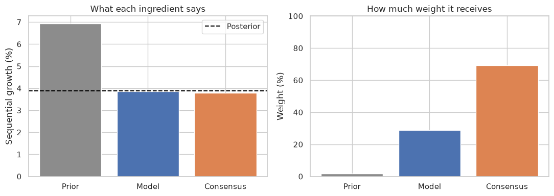
Growth readings and posterior weights for the three ingredients.
Figure 3: Estimated precision determines each weight.

7. Compare the answers in revenue units

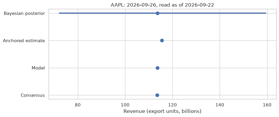
  • Anchored estimate: The frozen rule expresses expected surprise relative to consensus. Its intercept and revision term can place it outside the gap between the model and consensus.
  • Bayesian posterior: The independent precision-weighted combination operates in growth space and includes the historical prior as a third ingredient.
  • Interval: The displayed band uses the reference’s heavy-tailed Student-t settings. A broad interval exposes uncertainty; it is not evidence of measured 90% coverage on this company.
  • No winner inferred: This single example cannot establish which method is more accurate. That requires a separate, provenance-aware evaluation.
levels = pd.Series(
    {
        "Consensus": subjects.consensus.iloc[0],
        "Model": subjects.forecast.iloc[0],
        "Anchored estimate": anchored.anchored_level.iloc[0],
        "Bayesian posterior": posterior["prediction"],
    }
)
fig, ax = plt.subplots(figsize=(10, 4))
ax.scatter(levels / 1e9, levels.index, s=65, zorder=3)
ax.hlines(
    "Bayesian posterior",
    posterior["prediction-lower"] / 1e9,
    posterior["prediction-upper"] / 1e9,
    color=examples.ACCENT,
    linewidth=3,
)
ax.set(
    xlabel="Revenue (export units, billions)",
    title=f"{ticker}: {period}, read as of {as_of:%Y-%m-%d}",
)
plt.show()
Four revenue estimates and the Bayesian uncertainty interval.
Figure 4: Two methods applied to the same current readings.
levels.div(1e9).rename("Revenue (export units, billions)").round(3).to_frame()
Revenue (export units, billions)
Consensus 113.564
Model 113.644
Anchored estimate 115.464
Bayesian posterior 113.650

8. Inspect what cannot be published

Farther-out periods may have consensus but no live model. The output retains those subjects and their reasons. A diagnostic or a consensus value alone is not permission to treat a refused prediction as published.

Removing the live forecast demonstrates an anchored refusal on the same subject. The original calculation remains unchanged.

show(posteriors[["period", "prediction", "eligible", "eligibility_reason"]])
without_model = panel.loc[panel.source.ne("model")]
refused = pf.publish_anchored(
    without_model,
    as_of,
    forecast_source="model",
    parameters=parameters,
    subjects=subject_panel[
        ["entity", "period", "target", "period_end"]
    ].drop_duplicates(),
)
show(refused[["period", "expected_surprise", "eligible", "eligibility_reason"]])
period prediction eligible eligibility_reason
0 2026-09-26 1.136502e+11 True eligible
1 2026-12-26 1.503564e+11 True eligible
2 2027-03-27 NaN False insufficient_inputs_or_history
3 2027-06-26 NaN False insufficient_inputs_or_history
4 2027-09-25 NaN False insufficient_inputs_or_history
5 2028-01-01 NaN False insufficient_inputs_or_history
6 2028-04-01 NaN False insufficient_inputs_or_history
7 2028-07-01 NaN False insufficient_inputs_or_history
8 2028-09-30 NaN False insufficient_inputs_or_history
9 2028-12-30 NaN False insufficient_inputs_or_history
10 2029-03-31 NaN False insufficient_inputs_or_history
period expected_surprise eligible eligibility_reason
0 2026-09-26 NaN False missing_input

9. Check the calculation and keep the record

These executable checks verify the arithmetic and that filtering out observations at or after as_of leaves the Bayesian result unchanged. They cannot establish upstream historical availability; that requires the model and vendor provenance.

The audit payload records method settings and file hashes. Store it alongside the input snapshot and the exact installed postforecast revision in the consuming application.

np.testing.assert_allclose(contributions.sum(), anchored.expected_surprise.iloc[0])
np.testing.assert_allclose(ingredients.Weight.sum(), 1.0)
np.testing.assert_allclose(
    ingredients["Weighted growth"].sum(), posterior["posterior-growth"]
)
np.testing.assert_equal(bool(snapshot.known_at.lt(as_of).all()), desired=True)
np.testing.assert_equal(bool(refused.eligible.any()), desired=False)
np.testing.assert_equal(bool(refused.expected_surprise.isna().all()), desired=True)
trimmed = pf.bayesian_kpi_predictions(
    panel.loc[panel.known_at.lt(as_of)],
    as_of,
    forecast_source="model",
    backtest_source="model_history",
    settings=settings,
)
pd.testing.assert_frame_equal(posteriors, trimmed)
audit_record = {
    "export": export_root.name,
    "entity": entity,
    "period": period,
    "as_of": as_of.isoformat(),
    "source_files": provenance,
    "anchoring": anchoring.to_dict(),
    "bayesian": settings.model_dump(mode="json"),
}
print("Checks passed: attribution, weights, posterior, cutoff, and refusal.")
Checks passed: attribution, weights, posterior, cutoff, and refusal.

Try the methodology yourself

  1. Move the reading moment: Choose an earlier as_of within the live-model coverage and rerun. Observe which timestamps are selected and whether the freshness rules still permit publication.
  2. Change the target: Use another fiscal period visible in the output. Keep all historical input periods so the posterior retains its training history.
  3. Raise the history threshold: Increase minimum_observations and inspect eligibility, missing weights, and intervals. The independent reference has a documented forward two-way update when model precision is unavailable; read that rule before interpreting such a result.
  4. Inspect a different model: Change the ticker and select a matching fiscal period. Confirm coverage and units before comparing the result.
  5. Go deeper: Follow Anchoring, Bayesian posterior, and the correlation-adjusted reference.

A production caller additionally decides which export vintage, source freshness policy, parameter calibration, and interval validation are appropriate for its use. The Bayesian API does not inherit the anchored method’s age limits automatically.